Circular uniform distribution

In probability theory and directional statistics, a circular uniform distribution is a probability distribution on the unit circle whose density is uniform for all angles.

Description

Definition

The probability density function (pdf) of the circular uniform distribution, e.g. with ${\displaystyle \theta \in [0,2\pi )}$, is:

${\displaystyle f_{UC}(\theta )={\frac {1}{2\pi }}.}$

Moments with respect to a parametrization

We consider the circular variable ${\displaystyle z=e^{i\theta }}$ with ${\displaystyle z=1}$ at base angle ${\displaystyle \theta =0}$. In these terms, the circular moments of the circular uniform distribution are all zero, except for ${\displaystyle m_{0}}$:

${\displaystyle \langle z^{n}\rangle =\delta _{n}}$

where ${\displaystyle \delta _{n}}$ is the Kronecker delta symbol.

Descriptive statistics

Here the mean angle is undefined, and the length of the mean resultant is zero.

${\displaystyle R=|\langle z^{n}\rangle |=0\,}$

Distribution of the mean

The sample mean of a set of N measurements ${\displaystyle z_{n}=e^{i\theta _{n}}}$ drawn from a circular uniform distribution is defined as:

${\displaystyle {\overline {z}}={\frac {1}{N}}\sum _{n=1}^{N}z_{n}={\overline {C}}+i{\overline {S}}={\overline {R}}e^{i{\overline {\theta }}}}$

where the average sine and cosine are:^[1]

${\displaystyle {\overline {C}}={\frac {1}{N}}\sum _{n=1}^{N}\cos(\theta _{n})\qquad \qquad {\overline {S}}={\frac {1}{N}}\sum _{n=1}^{N}\sin(\theta _{n})}$

and the average resultant length is:

${\displaystyle {\overline {R}}^{2}=|{\overline {z}}|^{2}={\overline {C}}^{2}+{\overline {S}}^{2}}$

and the mean angle is:

${\displaystyle {\overline {\theta }}=\mathrm {Arg} ({\overline {z}}).\,}$

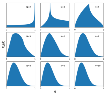
The sample mean for the circular uniform distribution will be concentrated about zero, becoming more concentrated as N increases. The distribution of the sample mean for the uniform distribution is given by:^[2]

${\displaystyle {\frac {1}{(2\pi )^{N}}}\int _{\Gamma }\prod _{n=1}^{N}d\theta _{n}=P({\overline {R}})P({\overline {\theta }})\,d{\overline {R}}\,d{\overline {\theta }}}$

where ${\displaystyle \Gamma \,}$ consists of intervals of ${\displaystyle 2\pi }$ in the variables, subject to the constraint that ${\displaystyle {\overline {R}}}$ and ${\displaystyle {\overline {\theta }}}$ are constant, or, alternatively, that ${\displaystyle {\overline {C}}}$ and ${\displaystyle {\overline {S}}}$ are constant. The distribution of the angle${\displaystyle P({\overline {\theta }})}$ is uniform

${\displaystyle P({\overline {\theta }})={\frac {1}{2\pi }}}$

and the distribution of ${\displaystyle {\overline {R}}}$ is given by:^[2]

${\displaystyle P_{N}({\overline {R}})=N^{2}{\overline {R}}\int _{0}^{\infty }J_{0}(N{\overline {R}}\,t)J_{0}(t)^{N}t\,dt}$

where ${\displaystyle J_{0}}$ is the Bessel function of order zero. There is no known general analytic solution for the above integral, and it is difficult to evaluate due to the large number of oscillations in the integrand. A 10,000 point Monte Carlo simulation of the distribution of the mean for N=3 is shown in the figure.

For certain special cases, the above integral can be evaluated:

${\displaystyle P_{2}({\overline {R}})={\frac {2}{\pi {\sqrt {1-{\overline {R}}^{2}}}}}.}$

For large N, the distribution of the mean can be determined from the central limit theorem for directional statistics. Since the angles are uniformly distributed, the individual sines and cosines of the angles will be distributed as:

${\displaystyle P(u)du={\frac {1}{\pi }}\,{\frac {du}{\sqrt {1-u^{2}}}}}$

where ${\displaystyle u=\cos \theta _{n}\,}$ or ${\displaystyle \sin \theta _{n}\,}$. It follows that they will have zero mean and a variance of 1/2. By the central limit theorem, in the limit of large N, ${\displaystyle {\overline {C}}\,}$ and ${\displaystyle {\overline {S}}\,}$, being the sum of a large number of i.i.d's, will be normally distributed with mean zero and variance ${\displaystyle 1/2N}$. The mean resultant length ${\displaystyle {\overline {R}}\,}$, being the square root of the sum of squares of two normally distributed independent variables, will be Chi-distributed with two degrees of freedom (i.e.Rayleigh-distributed) and variance ${\displaystyle 1/2N}$:

${\displaystyle \lim _{N\rightarrow \infty }P_{N}({\overline {R}})=2N{\overline {R}}\,e^{-N{\overline {R}}^{2}}.}$

Entropy

The differential information entropy of the uniform distribution is simply

${\displaystyle H_{U}=-\int _{\Gamma }{\frac {1}{2\pi }}\ln \left({\frac {1}{2\pi }}\right)\,d\theta =\ln(2\pi )}$

where ${\displaystyle \Gamma }$ is any interval of length ${\displaystyle 2\pi }$. This is the maximum entropy any circular distribution may have.

See also

• Wrapped distribution

References