Stirling number
Important sequences in combinatorics
In mathematics, Stirling numbers arise in a variety of analytic and combinatorial problems. They are named after James Stirling, who introduced them in a purely algebraic setting in his book Methodus differentialis (1730).[1] They were rediscovered and given a combinatorial meaning by Masanobu Saka in 1782.[2]
Two different sets of numbers bear this name: the Stirling numbers of the first kind and the Stirling numbers of the second kind. Additionally, Lah numbers are sometimes referred to as Stirling numbers of the third kind. Each kind is detailed in its respective article, this one serving as a description of relations between them.
A common property of all three kinds is that they describe coefficients relating three different sequences of polynomials that frequently arise in combinatorics. Moreover, all three can be defined as the number of partitions of n elements into k non-empty subsets, where each subset is endowed with a certain kind of order (no order, cyclical, or linear).
Notation
Several different notations for Stirling numbers are in use. Ordinary (signed) Stirling numbers of the first kind are commonly denoted:

Unsigned Stirling numbers of the first kind, which count the number of permutations of n elements with k disjoint cycles, are denoted:
![{\displaystyle {\biggl [}{n \atop k}{\biggr ]}=c(n,k)=|s(n,k)|=(-1)^{n-k}s(n,k)\,}](https://wikimedia.org/api/rest_v1/media/math/render/svg/ff56ff0a1f39d29c4fdb9e43faf74d13818fbd34)
Stirling numbers of the second kind, which count the number of ways to partition a set of n elements into k nonempty subsets:[3]

Abramowitz and Stegun use an uppercase and a blackletter , respectively, for the first and second kinds of Stirling number. The notation of brackets and braces, in analogy to binomial coefficients, was introduced in 1935 by Jovan Karamata and promoted later by Donald Knuth. (The bracket notation conflicts with a common notation for Gaussian coefficients.[4]) The mathematical motivation for this type of notation, as well as additional Stirling number formulae, may be found on the page for Stirling numbers and exponential generating functions.


Another infrequent notation is and .


Expansions of falling and rising factorials
Stirling numbers express coefficients in expansions of falling and rising factorials (also known as the Pochhammer symbol) as polynomials.
That is, the falling factorial, defined as is a polynomial in x of degree n whose expansion is


with (signed) Stirling numbers of the first kind as coefficients.
Note that by convention, because it is an empty product. The notations for the falling factorial and for the rising factorial are also often used.[5] (Confusingly, the Pochhammer symbol that many use for falling factorials is used in special functions for rising factorials.)


Similarly, the rising factorial, defined as is a polynomial in x of degree n whose expansion is

![{\displaystyle x^{(n)}\ =\ \sum _{k=0}^{n}\ {\biggl [}{n \atop k}{\biggr ]}\ x^{k}\ =\ \sum _{k=0}^{n}\ (-1)^{n-k}\ s(n,k)\ x^{k}\ ,}](https://wikimedia.org/api/rest_v1/media/math/render/svg/ee5872df65edaf1c6a66b8ae2796137048cfceba)
with unsigned Stirling numbers of the first kind as coefficients. One of these expansions can be derived from the other by observing that

Stirling numbers of the second kind express the reverse relations:

and

As change of basis coefficients
Considering the set of polynomials in the (indeterminate) variable x as a vector space, each of the three sequences

is a basis. That is, every polynomial in x can be written as a sum for some unique coefficients (similarly for the other two bases). The above relations then express the change of basis between them, as summarized in the following commutative diagram:


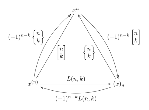
A diagram of how different Stirling numbers give coefficients for changing one basis of polynomials to another

The coefficients for the two bottom changes are described by the Lah numbers below. Since coefficients in any basis are unique, one can define Stirling numbers this way, as the coefficients expressing polynomials of one basis in terms of another, that is, the unique numbers relating with falling and rising factorials as above.

Falling factorials define, up to scaling, the same polynomials as binomial coefficients: . The changes between the standard basis and the basis are thus described by similar formulas:


- .

Example
Expressing a polynomial in the basis of falling factorials is useful for calculating sums of the polynomial evaluated at consecutive integers. Indeed, the sum of falling factorials with fixed k can expressed as another falling factorial (for )


This can be proved by induction.
For example, the sum of fourth powers of integers up to n (this time with n included), is:
![{\displaystyle {\begin{aligned}\sum _{i=0}^{n}i^{4}&=\sum _{i=0}^{n}\sum _{k=0}^{4}{\biggl \{}{\!4\! \atop \!k\!}{\biggr \}}(i)_{k}=\sum _{k=0}^{4}{\biggl \{}{\!4\! \atop \!k\!}{\biggr \}}\sum _{i=0}^{n}(i)_{k}=\sum _{k=0}^{4}{\biggl \{}{\!4\! \atop \!k\!}{\biggr \}}{\frac {(n{+}1)_{k+1}}{k{+}1}}\\[10mu]&={\biggl \{}{\!4\! \atop \!1\!}{\biggr \}}{\frac {(n{+}1)_{2}}{2}}+{\biggl \{}{\!4\! \atop \!2\!}{\biggr \}}{\frac {(n{+}1)_{3}}{3}}+{\biggl \{}{\!4\! \atop \!3\!}{\biggr \}}{\frac {(n{+}1)_{4}}{4}}+{\biggl \{}{\!4\! \atop \!4\!}{\biggr \}}{\frac {(n{+}1)_{5}}{5}}\\[8mu]&={\frac {1}{2}}(n{+}1)_{2}+{\frac {7}{3}}(n{+}1)_{3}+{\frac {6}{4}}(n{+}1)_{4}+{\frac {1}{5}}(n{+}1)_{5}\,.\end{aligned}}}](https://wikimedia.org/api/rest_v1/media/math/render/svg/0ae77860888a00722dde0d01f031c9d189ddae65)
Here the Stirling numbers can be computed from their definition as the number of partitions of 4 elements into k non-empty unlabeled subsets.
In contrast, the sum in the standard basis is given by Faulhaber's formula, which in general is more complicated.

As inverse matrices
The Stirling numbers of the first and second kinds can be considered inverses of one another:
![{\displaystyle \sum _{j=k}^{n}s(n,j)S(j,k)=\sum _{j=k}^{n}(-1)^{n-j}{\biggl [}{n \atop j}{\biggr ]}{\biggl \{}{\!j\! \atop \!k\!}{\biggr \}}=\delta _{n,k}}](https://wikimedia.org/api/rest_v1/media/math/render/svg/d866c838f784a76038bc6835d191d0a428fa703f)
and
![{\displaystyle \sum _{j=k}^{n}S(n,j)s(j,k)=\sum _{j=k}^{n}(-1)^{j-k}{\biggl \{}{\!n\! \atop \!j\!}{\biggr \}}{\biggl [}{j \atop k}{\biggr ]}=\delta _{n,k},}](https://wikimedia.org/api/rest_v1/media/math/render/svg/00a0a9383d73081a147f80c791b4cbfbbad44eef)
where is the Kronecker delta. These two relationships may be understood to be matrix inverse relationships. That is, let s be the lower triangular matrix of Stirling numbers of the first kind, whose matrix elements The inverse of this matrix is S, the lower triangular matrix of Stirling numbers of the second kind, whose entries are Symbolically, this is written


Although s and S are infinite, so calculating a product entry involves an infinite sum, the matrix multiplications work because these matrices are lower triangular, so only a finite number of terms in the sum are nonzero.
Lah numbers
The Lah numbers are sometimes called Stirling numbers of the third kind.[6] By convention, and if or .


These numbers are coefficients expressing falling factorials in terms of rising factorials and vice versa:
- and


As above, this means they express the change of basis between the bases and , completing the diagram. In particular, one formula is the inverse of the other, thus:


Similarly, composing the change of basis from to with the change of basis from to gives the change of basis directly from to :


![{\displaystyle L(n,k)=\sum _{j=k}^{n}{\biggl [}{n \atop j}{\biggr ]}{\biggl \{}{\!j\! \atop \!k\!}{\biggr \}},}](https://wikimedia.org/api/rest_v1/media/math/render/svg/ce67f09dcebbc9f778fde72e43f31696e49d2f40)
and similarly for other compositions. In terms of matrices, if denotes the matrix with entries and denotes the matrix with entries , then one is the inverse of the other: . Composing the matrix of unsigned Stirling numbers of the first kind with the matrix of Stirling numbers of the second kind gives the Lah numbers: .


Enumeratively, can be defined as the number of partitions of n elements into k non-empty unlabeled subsets, where each subset is endowed with no order, a cyclic order, or a linear order, respectively. In particular, this implies the inequalities:
![{\textstyle \left\{{\!n\! \atop \!k\!}\right\},\left[{n \atop k}\right],L(n,k)}](https://wikimedia.org/api/rest_v1/media/math/render/svg/dc26eedaa94e5b7e121762310ad713db0b92b2e3)
![{\displaystyle {\biggl \{}{\!n\! \atop \!k\!}{\biggr \}}\leq {\biggl [}{n \atop k}{\biggr ]}\leq L(n,k).}](https://wikimedia.org/api/rest_v1/media/math/render/svg/df78c5212ed960b65aed0ba87be0ca3eefdd293c)
Inversion relations and the Stirling transform
For any pair of sequences, and , related by a finite sum Stirling number formula given by


for all integers , we have a corresponding inversion formula for given by


^{n-k}g_{k}.}](https://wikimedia.org/api/rest_v1/media/math/render/svg/cf0de636ecc3989622d39a0e7eb8c91859991778)
The lower indices could be any integer between and .


These inversion relations between the two sequences translate into functional equations between the sequence exponential generating functions given by the Stirling (generating function) transform as

and

For , the differential operators and are related by the following formulas for all integers :[7]


Another pair of "inversion" relations involving the Stirling numbers relate the forward differences and the ordinary derivatives of a function, , which is analytic for all by the formulas[8]


Similar properties
| Stirling numbers of the first kind | Stirling numbers of the second kind |
|---|---|
| , where is the n-th Bell number | |
| , where is the rising factorials | , where is the Touchard polynomials |
![{\displaystyle \left[{n+1 \atop k}\right]=n\left[{n \atop k}\right]+\left[{n \atop k-1}\right]}](https://wikimedia.org/api/rest_v1/media/math/render/svg/406f793535c38a92fa1ebfc14cb382a1e0be0fdf)

![{\displaystyle \sum _{k=0}^{n}\left[{n \atop k}\right]=n!}](https://wikimedia.org/api/rest_v1/media/math/render/svg/7b3d2ba78741f8131184b255a1b4b746c6e639a2)


![{\displaystyle \sum _{k=0}^{n}\left[{n \atop k}\right]x^{k}=x^{(n)}}](https://wikimedia.org/api/rest_v1/media/math/render/svg/c2ea08e773efe86193183bbdb1cc82e0d7af965d)


![{\displaystyle \left[{n \atop 0}\right]=\delta _{n},\ \left[{n \atop n-1}\right]={\binom {n}{2}},\ \left[{n \atop n}\right]=1}](https://wikimedia.org/api/rest_v1/media/math/render/svg/a279a1e5a3d0a8ca253cac9d5adb55c08bfc5bc8)

![{\displaystyle \left[{n+1 \atop k+1}\right]=\sum _{j=k}^{n}\left[{n \atop j}\right]{\binom {j}{k}}}](https://wikimedia.org/api/rest_v1/media/math/render/svg/7bcc7526ee57ac883ee131a7ac47cb74969baf5d)

![{\displaystyle \left[{\begin{matrix}n+1\\k+1\end{matrix}}\right]=\sum _{j=k}^{n}{\frac {n!}{j!}}\left[{j \atop k}\right]}](https://wikimedia.org/api/rest_v1/media/math/render/svg/058551fa500507f041172138eaac96abc478781f)

![{\displaystyle \left[{n+k+1 \atop n}\right]=\sum _{j=0}^{k}(n+j)\left[{n+j \atop j}\right]}](https://wikimedia.org/api/rest_v1/media/math/render/svg/c847a76190ef97fea7180a8c32bf1ed76eab902a)

![{\displaystyle \left[{n \atop l+m}\right]{\binom {l+m}{l}}=\sum _{k}\left[{k \atop l}\right]\left[{n-k \atop m}\right]{\binom {n}{k}}}](https://wikimedia.org/api/rest_v1/media/math/render/svg/51534e1ae519abc7d8f3fdd386dade48db83ff98)

![{\displaystyle \left[{n+k \atop n}\right]{\underset {n\to \infty }{\sim }}{\frac {n^{2k}}{2^{k}k!}}.}](https://wikimedia.org/api/rest_v1/media/math/render/svg/442b6da76d0fc5aec61273a78af3d8c7142075ed)

![{\displaystyle \sum _{n=k}^{\infty }\left[{n \atop k}\right]{\frac {x^{n}}{n!}}={\frac {(-\log(1-x))^{k}}{k!}}.}](https://wikimedia.org/api/rest_v1/media/math/render/svg/138bd8f306691ce66b23b2c01c94afc42f5f4a90)

![{\displaystyle \left[{n \atop k}\right]=\sum _{0\leq i_{1}<\ldots <i_{n-k}<n}i_{1}i_{2}\cdots i_{n-k}.}](https://wikimedia.org/api/rest_v1/media/math/render/svg/de97ae70a1f565b4eb9fa5d703e5d0fbdcea6dff)

See the specific articles for details.
Symmetric formulae
Abramowitz and Stegun give the following symmetric formulae that relate the Stirling numbers of the first and second kind.[9]
![{\displaystyle \left[{n \atop k}\right]=\sum _{j=n}^{2n-k}(-1)^{j-k}{\binom {j-1}{k-1}}{\binom {2n-k}{j}}\left\{{j-k \atop j-n}\right\}}](https://wikimedia.org/api/rest_v1/media/math/render/svg/55b396b7588b8b75ad99d03868f7aa1eadbb5c5b)
and
![{\displaystyle \left\{{n \atop k}\right\}=\sum _{j=n}^{2n-k}(-1)^{j-k}{\binom {j-1}{k-1}}{\binom {2n-k}{j}}\left[{j-k \atop j-n}\right]}](https://wikimedia.org/api/rest_v1/media/math/render/svg/4b536640328c88e08cf7a068aeb47c3a77c7d5e8)
Stirling numbers with negative integral values
The Stirling numbers can be extended to negative integral values, but not all authors do so in the same way.[10][11][12] Regardless of the approach taken, it is worth noting that Stirling numbers of first and second kind are connected by the relations:
![{\displaystyle {\biggl [}{n \atop k}{\biggr ]}={\biggl \{}{\!-k\! \atop \!-n\!}{\biggr \}}\quad {\text{and}}\quad {\biggl \{}{\!n\! \atop \!k\!}{\biggr \}}={\biggl [}{-k \atop -n}{\biggr ]}}](https://wikimedia.org/api/rest_v1/media/math/render/svg/e9f12872029952e3a00f2a2e6cff8da907b5c372)
when n and k are nonnegative integers. So we have the following table for :
![{\displaystyle \left[{-n \atop -k}\right]}](https://wikimedia.org/api/rest_v1/media/math/render/svg/d4b082da53ea89c6b9e736335552cceb8ed6069e)
k n | −1 | −2 | −3 | −4 | −5 |
|---|---|---|---|---|---|
| −1 | 1 | 1 | 1 | 1 | 1 |
| −2 | 0 | 1 | 3 | 7 | 15 |
| −3 | 0 | 0 | 1 | 6 | 25 |
| −4 | 0 | 0 | 0 | 1 | 10 |
| −5 | 0 | 0 | 0 | 0 | 1 |
Donald Knuth[12] defined the more general Stirling numbers by extending a recurrence relation to all integers. In this approach, and are zero if n is negative and k is nonnegative, or if n is nonnegative and k is negative, and so we have, for any integers n and k,
![{\textstyle \left[{n \atop k}\right]}](https://wikimedia.org/api/rest_v1/media/math/render/svg/0eda457849a3bdae75a608661a9520cae5ce8a6c)

![{\displaystyle {\biggl [}{n \atop k}{\biggr ]}={\biggl \{}{\!-k\! \atop \!-n\!}{\biggr \}}\quad {\text{and}}\quad {\biggl \{}{\!n\! \atop \!k\!}{\biggr \}}={\biggl [}{-k \atop -n}{\biggr ]}.}](https://wikimedia.org/api/rest_v1/media/math/render/svg/0b03ad1a4792348c1acf9f5ef46b70b35687264f)
On the other hand, for positive integers n and k, David Branson[11] defined and (but not or ). In this approach, one has the following extension of the recurrence relation of the Stirling numbers of the first kind:
![{\textstyle \left[{-n \atop -k}\right]\!,}](https://wikimedia.org/api/rest_v1/media/math/render/svg/2e5922f6d16f68a5c91afc67a34cece3be89fc24)

![{\textstyle \left[{-n \atop k}\right]\!,}](https://wikimedia.org/api/rest_v1/media/math/render/svg/8e115fa99ba4cc0fff4c01ce6932201079e4dc3e)

![{\textstyle \left[{n \atop -k}\right]}](https://wikimedia.org/api/rest_v1/media/math/render/svg/c8da0d6e5d3f6db3106312f622e6d954b1f65070)

- ,
![{\displaystyle {\biggl [}{-n \atop k}{\biggr ]}={\frac {(-1)^{n+1}}{n!}}\sum _{i=1}^{n}{\frac {(-1)^{i+1}}{i^{k}}}{\binom {n}{i}}}](https://wikimedia.org/api/rest_v1/media/math/render/svg/ffdb9afe821b203f793c2c8ba04aab0b713a296b)
For example, This leads to the following table of values of for negative integral n.
![{\textstyle \left[{-5 \atop k}\right]={\frac {1}{120}}{\Bigl (}5-{\frac {10}{2^{k}}}+{\frac {10}{3^{k}}}-{\frac {5}{4^{k}}}+{\frac {1}{5^{k}}}{\Bigr )}.}](https://wikimedia.org/api/rest_v1/media/math/render/svg/a92356fcae50ab1ac548ebe38fa6b1764e322699)
k n | 0 | 1 | 2 | 3 | 4 |
|---|---|---|---|---|---|
| −1 | 1 | 1 | 1 | 1 | 1 |
| −2 | |||||
| −3 | |||||
| −4 | |||||
| −5 |


In this case where is a Bell number, and so one may define the negative Bell numbers by .
![{\textstyle \sum _{n=1}^{\infty }\left[{-n \atop -k}\right]=B_{k}}](https://wikimedia.org/api/rest_v1/media/math/render/svg/900906e78c8883aa541b8798614bc2145bf4a72b)

![{\textstyle \sum _{n=1}^{\infty }\left[{-n \atop k}\right]=:B_{-k}}](https://wikimedia.org/api/rest_v1/media/math/render/svg/81cddaa2425275840e603da66b2f8f76bdd23fea)
For example, this produces , generally .
![{\textstyle \sum _{n=1}^{\infty }\left[{-n \atop 1}\right]=B_{-1}={\frac {1}{e}}\sum _{j=1}^{\infty }{\frac {1}{j\cdot j!}}={\frac {1}{e}}\int _{0}^{1}{\frac {e^{t}-1}{t}}dt=0.4848291\dots }](https://wikimedia.org/api/rest_v1/media/math/render/svg/4a13a7742887bd6a1555435cc16dd9f2326d5592)

See also
- Bell polynomials
- Catalan number
- Cycles and fixed points
- Pochhammer symbol
- Polynomial sequence
- Touchard polynomials
- Stirling permutation
Citations
- ^ Mansour & Schork 2015, p. 5.
- ^ Mansour & Schork 2015, p. 4.
- ^ Ronald L. Graham, Donald E. Knuth, Oren Patashnik (1988) Concrete Mathematics, Addison-Wesley, Reading MA. ISBN 0-201-14236-8, p. 244.
- ^ Donald Knuth
- ^ Aigner, Martin (2007). "Section 1.2 - Subsets and binomial coefficients". A Course in Enumeration. Springer. pp. 561. ISBN 978-3-540-39032-9.
- ^ Sándor, Jozsef; Crstici, Borislav (2004). Handbook of Number Theory II. Kluwer Academic Publishers. p. 464. ISBN 9781402025464.
- ^ Concrete Mathematics exercise 13 of section 6. Note that this formula immediately implies the first positive-order Stirling number transformation given in the main article on generating function transformations.
- ^ Olver, Frank; Lozier, Daniel; Boisvert, Ronald; Clark, Charles (2010). "NIST Handbook of Mathematical Functions". NIST Handbook of Mathematical Functions. (Section 26.8)
- ^ Goldberg, K.; Newman, M; Haynsworth, E. (1972), "Stirling Numbers of the First Kind, Stirling Numbers of the Second Kind", in Abramowitz, Milton; Stegun, Irene A. (eds.), Handbook of Mathematical Functions with Formulas, Graphs, and Mathematical Tables, 10th printing, New York: Dover, pp. 824–825
- ^ Loeb, Daniel E. (1992) [Received 3 Nov 1989]. "A generalization of the Stirling numbers". Discrete Mathematics. 103 (3): 259–269. doi:10.1016/0012-365X(92)90318-A.
- ^ a b Branson, David (August 1994). "An extension of Stirling numbers" (PDF). The Fibonacci Quarterly. Archived (PDF) from the original on 2011-08-27. Retrieved Dec 6, 2017.
- ^ a b D.E. Knuth, 1992.
References
- Rosen, Kenneth H., ed. (2018), Handbook of Discrete and Combinatorial Mathematics, CRC Press, ISBN 978-1-5848-8780-5
- Mansour, Toufik; Schork, Mathias (2015), Commutation Relations, Normal Ordering, and Stirling Numbers, CRC Press, ISBN 978-1-4665-7989-7
Further reading
- Adamchik, Victor (1997). "On Stirling Numbers and Euler Sums" (PDF). Journal of Computational and Applied Mathematics. 79: 119–130. doi:10.1016/s0377-0427(96)00167-7. Archived (PDF) from the original on 2004-12-14.
- Benjamin, Arthur T.; Preston, Gregory O.; Quinn, Jennifer J. (2002). "A Stirling Encounter with Harmonic Numbers" (PDF). Mathematics Magazine. 75 (2): 95–103. CiteSeerX 10.1.1.383.722. doi:10.2307/3219141. JSTOR 3219141. Archived (PDF) from the original on 2020-09-10.
- Boyadzhiev, Khristo N. (2012). "Close encounters with the Stirling numbers of the second kind" (PDF). Mathematics Magazine. 85 (4): 252–266. arXiv:1806.09468. doi:10.4169/math.mag.85.4.252. S2CID 115176876. Archived (PDF) from the original on 2015-09-05.
- Comtet, Louis (1970). "Valeur de s(n, k)". Analyse Combinatoire, Tome Second (in French): 51.
- Comtet, Louis (1974). Advanced Combinatorics: The Art of Finite and Infinite Expansions. Dordrecht-Holland/Boston-U.S.A.: Reidel Publishing Company. ISBN 9789027703804.
- Hsien-Kuei Hwang (1995). "Asymptotic Expansions for the Stirling Numbers of the First Kind". Journal of Combinatorial Theory, Series A. 71 (2): 343–351. doi:10.1016/0097-3165(95)90010-1.
- Knuth, D.E. (1992), "Two notes on notation", Amer. Math. Monthly, 99 (5): 403–422, arXiv:math/9205211, doi:10.2307/2325085, JSTOR 2325085, S2CID 119584305
- Miksa, Francis L. (January 1956). "Stirling numbers of the first kind: 27 leaves reproduced from typewritten manuscript on deposit in the UMT File". Mathematical Tables and Other Aids to Computation: Reviews and Descriptions of Tables and Books. 10 (53): 37–38. JSTOR 2002617.
- Miksa, Francis L. (1972) [1964]. "Combinatorial Analysis, Table 24.4, Stirling Numbers of the Second Kind". In Abramowitz, Milton; Stegun, Irene A. (eds.). Handbook of Mathematical Functions (with Formulas, Graphs and Mathematical Tables). 55. U.S. Dept. of Commerce, National Bureau of Standards, Applied Math. p. 835.
- Mitrinović, Dragoslav S. (1959). "Sur les nombres de Stirling de première espèce et les polynômes de Stirling" (PDF). Publications de la Faculté d'Electrotechnique de l'Université de Belgrade, Série Mathématiques et Physique (in French) (23): 1–20. ISSN 0522-8441. Archived (PDF) from the original on 2009-06-17.
- O'Connor, John J.; Robertson, Edmund F. (September 1998). "James Stirling (1692–1770)".
- Sixdeniers, J. M.; Penson, K. A.; Solomon, A. I. (2001). "Extended Bell and Stirling Numbers From Hypergeometric Exponentiation" (PDF). Journal of Integer Sequences. 4: 01.1.4. arXiv:math/0106123. Bibcode:2001JIntS...4...14S.
- Spivey, Michael Z. (2007). "Combinatorial sums and finite differences". Discrete Math. 307 (24): 3130–3146. CiteSeerX 10.1.1.134.8665. doi:10.1016/j.disc.2007.03.052.
- Sloane, N. J. A. (ed.). "Sequence A008275 (Stirling numbers of first kind)". The On-Line Encyclopedia of Integer Sequences. OEIS Foundation.
- Sloane, N. J. A. (ed.). "Sequence A008277 (Stirling numbers of 2nd kind)". The On-Line Encyclopedia of Integer Sequences. OEIS Foundation.
- v
- t
- e
Classes of natural numbers
Of the form a × 2b ± 1 | |
|---|---|
Other polynomial numbers | |
|---|---|
Recursively defined numbers | |
|---|---|
Possessing a specific set of other numbers | |
|---|---|
Expressible via specific sums | |
|---|---|
| |||||||||||||||||||
Combinatorial numbers | |
|---|---|
| |||||||||||
Numeral system-dependent numbers | |||||||||||||||||||||
|---|---|---|---|---|---|---|---|---|---|---|---|---|---|---|---|---|---|---|---|---|---|
| |||||||||||||||||||||
Generated via a sieve | |
|---|---|
 Mathematics portal


