Step function

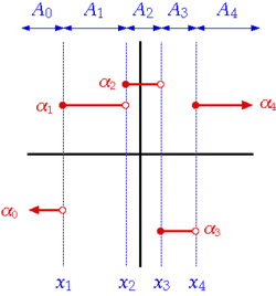
In mathematics, a function on the real numbers is called a step function if it can be written as a finite linear combination of indicator functions of intervals. Informally speaking, a step function is a piecewise constant function having only finitely many pieces.

Definition and first consequences

A function ${\displaystyle f\colon \mathbb {R} \rightarrow \mathbb {R} }$ is called a step function if it can be written as ^{[citation needed]}

${\displaystyle f(x)=\sum \limits _{i=0}^{n}\alpha _{i}\chi _{A_{i}}(x)}$, for all real numbers ${\displaystyle x}$

where ${\displaystyle n\geq 0}$, ${\displaystyle \alpha _{i}}$ are real numbers, ${\displaystyle A_{i}}$ are intervals, and ${\displaystyle \chi _{A}}$ is the indicator function of ${\displaystyle A}$:

${\displaystyle \chi _{A}(x)={\begin{cases}1&{\text{if }}x\in A\\0&{\text{if }}x\notin A\\\end{cases}}}$

In this definition, the intervals ${\displaystyle A_{i}}$ can be assumed to have the following two properties:

1. The intervals are pairwise disjoint: ${\displaystyle A_{i}\cap A_{j}=\emptyset }$ for ${\displaystyle i\neq j}$
2. The union of the intervals is the entire real line: ${\displaystyle \bigcup _{i=0}^{n}A_{i}=\mathbb {R} .}$

Indeed, if that is not the case to start with, a different set of intervals can be picked for which these assumptions hold. For example, the step function

${\displaystyle f=4\chi _{[-5,1)}+3\chi _{(0,6)}}$

can be written as

${\displaystyle f=0\chi _{(-\infty ,-5)}+4\chi _{[-5,0]}+7\chi _{(0,1)}+3\chi _{[1,6)}+0\chi _{[6,\infty )}.}$

Variations in the definition

Sometimes, the intervals are required to be right-open^[1] or allowed to be singleton.^[2] The condition that the collection of intervals must be finite is often dropped, especially in school mathematics,^[3][4][5] though it must still be locally finite, resulting in the definition of piecewise constant functions.

Examples

• A constant function is a trivial example of a step function. Then there is only one interval, ${\displaystyle A_{0}=\mathbb {R} .}$
• The sign function sgn(x), which is −1 for negative numbers and +1 for positive numbers, and is the simplest non-constant step function.
• The Heaviside function H(x), which is 0 for negative numbers and 1 for positive numbers, is equivalent to the sign function, up to a shift and scale of range (${\displaystyle H=(\operatorname {sgn} +1)/2}$). It is the mathematical concept behind some test signals, such as those used to determine the step response of a dynamical system.

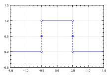
• The rectangular function, the normalized boxcar function, is used to model a unit pulse.

Non-examples

• The integer part function is not a step function according to the definition of this article, since it has an infinite number of intervals. However, some authors^[6] also define step functions with an infinite number of intervals.^[6]

Properties

• The sum and product of two step functions is again a step function. The product of a step function with a number is also a step function. As such, the step functions form an algebra over the real numbers.
• A step function takes only a finite number of values. If the intervals ${\displaystyle A_{i},}$ for ${\displaystyle i=0,1,\dots ,n}$ in the above definition of the step function are disjoint and their union is the real line, then ${\displaystyle f(x)=\alpha _{i}}$ for all ${\displaystyle x\in A_{i}.}$
• The definite integral of a step function is a piecewise linear function.
• The Lebesgue integral of a step function ${\displaystyle \textstyle f=\sum _{i=0}^{n}\alpha _{i}\chi _{A_{i}}}$ is ${\displaystyle \textstyle \int f\,dx=\sum _{i=0}^{n}\alpha _{i}\ell (A_{i}),}$ where ${\displaystyle \ell (A)}$ is the length of the interval ${\displaystyle A}$, and it is assumed here that all intervals ${\displaystyle A_{i}}$ have finite length. In fact, this equality (viewed as a definition) can be the first step in constructing the Lebesgue integral.^[7]
• A discrete random variable is sometimes defined as a random variable whose cumulative distribution function is piecewise constant.^[8] In this case, it is locally a step function (globally, it may have an infinite number of steps). Usually however, any random variable with only countably many possible values is called a discrete random variable, in this case their cumulative distribution function is not necessarily locally a step function, as infinitely many intervals can accumulate in a finite region.

See also

• Crenel function
• Piecewise
• Sigmoid function
• Simple function
• Step detection
• Heaviside step function
• Piecewise-constant valuation

References