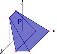
A 3-dimensional convex polytope. Convex analysis includes not only the study of convex subsets of Euclidean spaces but also the study of convex functions on abstract spaces.
Convex analysis is the branch of mathematics devoted to the study of properties of convex functions and convex sets, often with applications in convex minimization, a subdomain of optimization theory.
Convex sets
A subset of some vector space is convex if it satisfies any of the following equivalent conditions:
Throughout, will be a map valued in the extended real numbers with a domain that is a convex subset of some vector space. The map is a convex function if
(Convexity ≤)
holds for any real and any with If this remains true of when the defining inequality (Convexity ≤) is replaced by the strict inequality
Convex functions are related to convex sets. Specifically, the function is convex if and only if its epigraph
A function (in black) is convex if and only if its epigraph, which is the region above its graph (in green), is a convex set.A graph of the bivariate convex function
(Epigraph def.)
is a convex set.[2] The epigraphs of extended real-valued functions play a role in convex analysis that is analogous to the role played by graphs of real-valued function in real analysis. Specifically, the epigraph of an extended real-valued function provides geometric intuition that can be used to help formula or prove conjectures.
The domain of a function is denoted by while its effective domain is the set[2]
(dom f def.)
The function is called proper if and for all[2] Alternatively, this means that there exists some in the domain of at which and is also never equal to In words, a function is proper if its domain is not empty, it never takes on the value and it also is not identically equal to If is a proper convex function then there exist some vector and some such that
for every
where denotes the dot product of these vectors.
Convex conjugate
The convex conjugate of an extended real-valued function (not necessarily convex) is the function from the (continuous) dual space of and[3]
where the brackets denote the canonical duality The biconjugate of is the map defined by for every If denotes the set of -valued functions on then the map defined by is called the Legendre-Fenchel transform.
Subdifferential set and the Fenchel-Young inequality
If and then the subdifferential set is
For example, in the important special case where is a norm on , it can be shown[proof 1] that if then this definition reduces down to:
and
For any and which is called the Fenchel-Young inequality. This inequality is an equality (i.e. ) if and only if It is in this way that the subdifferential set is directly related to the convex conjugate
Biconjugate
The biconjugate of a function is the conjugate of the conjugate, typically written as The biconjugate is useful for showing when strong or weak duality hold (via the perturbation function).
A convex minimization (primal) problem is one of the form
find when given a convex function and a convex subset
Dual problem
In optimization theory, the duality principle states that optimization problems may be viewed from either of two perspectives, the primal problem or the dual problem.
If there are constraint conditions, these can be built into the function by letting where is the indicator function. Then let be a perturbation function such that [5]
The dual problem with respect to the chosen perturbation function is given by
where is the convex conjugate in both variables of
The duality gap is the difference of the right and left hand sides of the inequality[6][5][7]
This principle is the same as weak duality. If the two sides are equal to each other, then the problem is said to satisfy strong duality.
There are many conditions for strong duality to hold such as:
^Borwein, Jonathan; Lewis, Adrian (2006). Convex Analysis and Nonlinear Optimization: Theory and Examples (2 ed.). Springer. pp. 76–77. ISBN 978-0-387-29570-1.
^ abBoţ, Radu Ioan; Wanka, Gert; Grad, Sorin-Mihai (2009). Duality in Vector Optimization. Springer. ISBN 978-3-642-02885-4.
^Csetnek, Ernö Robert (2010). Overcoming the failure of the classical generalized interior-point regularity conditions in convex optimization. Applications of the duality theory to enlargements of maximal monotone operators. Logos Verlag Berlin GmbH. ISBN 978-3-8325-2503-3.
^Borwein, Jonathan; Lewis, Adrian (2006). Convex Analysis and Nonlinear Optimization: Theory and Examples (2 ed.). Springer. ISBN 978-0-387-29570-1.
^Boyd, Stephen; Vandenberghe, Lieven (2004). Convex Optimization(PDF). Cambridge University Press. ISBN 978-0-521-83378-3. Retrieved October 3, 2011.
^The conclusion is immediate if so assume otherwise. Fix Replacing with the norm gives If and is real then using gives where in particular, taking gives while taking gives and thus ; moreover, if in addition then because it follows from the definition of the dual norm that Because which is equivalent to it follows that which implies for all From these facts, the conclusion can now be reached. ∎
References
Bauschke, Heinz H.; Combettes, Patrick L. (28 February 2017). Convex Analysis and Monotone Operator Theory in Hilbert Spaces. CMS Books in Mathematics. Springer Science & Business Media. ISBN 978-3-319-48311-5. OCLC 1037059594.
Boyd, Stephen; Vandenberghe, Lieven (8 March 2004). Convex Optimization. Cambridge Series in Statistical and Probabilistic Mathematics. Cambridge, U.K. New York: Cambridge University Press. ISBN 978-0-521-83378-3. OCLC 53331084.
Hiriart-Urruty, J.-B.; Lemaréchal, C. (2001). Fundamentals of convex analysis. Berlin: Springer-Verlag. ISBN 978-3-540-42205-1.
Kusraev, A.G.; Kutateladze, Semen Samsonovich (1995). Subdifferentials: Theory and Applications. Dordrecht: Kluwer Academic Publishers. ISBN 978-94-011-0265-0.
Rudin, Walter (1991). Functional Analysis. International Series in Pure and Applied Mathematics. Vol. 8 (Second ed.). New York, NY: McGraw-Hill Science/Engineering/Math. ISBN 978-0-07-054236-5. OCLC 21163277.
Singer, Ivan (1997). Abstract convex analysis. Canadian Mathematical Society series of monographs and advanced texts. New York: John Wiley & Sons, Inc. pp. xxii+491. ISBN 0-471-16015-6. MR 1461544.
Stoer, J.; Witzgall, C. (1970). Convexity and optimization in finite dimensions. Vol. 1. Berlin: Springer. ISBN 978-0-387-04835-2.
Zălinescu, Constantin (30 July 2002). Convex Analysis in General Vector Spaces. River Edge, N.J. London: World Scientific Publishing. ISBN 978-981-4488-15-0. MR 1921556. OCLC 285163112 – via Internet Archive.
External links
Media related to Convex analysis at Wikimedia Commons


![{\displaystyle f:X\to [-\infty ,\infty ]}](https://wikimedia.org/api/rest_v1/media/math/render/svg/cb5b80b60f448c0542dc59fd71f22b8ce01e8bc7)
![{\displaystyle [-\infty ,\infty ]=\mathbb {R} \cup \{\pm \infty \}}](https://wikimedia.org/api/rest_v1/media/math/render/svg/f784980f597dae36b4d32c2a89de0a449e99aca8)


![{\displaystyle f:\mathbb {R} ^{n}\to [-\infty ,\infty ]}](https://wikimedia.org/api/rest_v1/media/math/render/svg/3ef5a82ad74366531ce71d6fe571255b18f1d29a)


![{\displaystyle f^{*}:X^{*}\to [-\infty ,\infty ]}](https://wikimedia.org/api/rest_v1/media/math/render/svg/1e13a90d630d56ab231b9102f8c606db82843f54)


![{\displaystyle f^{**}=\left(f^{*}\right)^{*}:X\to [-\infty ,\infty ]}](https://wikimedia.org/api/rest_v1/media/math/render/svg/3229c63ee01e8790a85b9f288eddca1b70746688)


![{\displaystyle \operatorname {Func} (X;[-\infty ,\infty ])\to \operatorname {Func} \left(X^{*};[-\infty ,\infty ]\right)}](https://wikimedia.org/api/rest_v1/media/math/render/svg/3e960704508725beb4b9514813c473cbdf955b5a)


![{\displaystyle f^{**}:X\to [-\infty ,\infty ].}](https://wikimedia.org/api/rest_v1/media/math/render/svg/074b6459bfe16e76142cf5bf8aadfb2282a86cb8)


![{\displaystyle f:X\to [-\infty ,\infty ],}](https://wikimedia.org/api/rest_v1/media/math/render/svg/40734dee6b4c8857e310c774d3d9a55acd73fff2)


![{\displaystyle F:X\times Y\to [-\infty ,\infty ]}](https://wikimedia.org/api/rest_v1/media/math/render/svg/4be0d8959e1b20e3299c0b75df57a15d0b809378)


![{\displaystyle \left\langle x^{*},x\right\rangle -\|x\|\geq \left\langle x^{*},rx\right\rangle -\|rx\|=r\left[\left\langle x^{*},x\right\rangle -\|x\|\right],}](https://wikimedia.org/api/rest_v1/media/math/render/svg/1204d83ef8154fa2d3b747047d2804e35743fab1)


 Media related to Convex analysis at Wikimedia Commons


