Anger function

Plot of the Anger function J v(z) with n=2 in the complex plane from -2-2i to 2+2i with colors created with Mathematica 13.1 function ComplexPlot3D

In mathematics, the Anger function, introduced by C. T. Anger (1855), is a function defined as

J ν ( z ) = 1 π 0 π cos ( ν θ z sin θ ) d θ {\displaystyle \mathbf {J} _{\nu }(z)={\frac {1}{\pi }}\int _{0}^{\pi }\cos(\nu \theta -z\sin \theta )\,d\theta }

with complex parameter ν {\displaystyle \nu } and complex variable z {\displaystyle {\textit {z}}} .[1] It is closely related to the Bessel functions.

The Weber function (also known as Lommel–Weber function), introduced by H. F. Weber (1879), is a closely related function defined by

E ν ( z ) = 1 π 0 π sin ( ν θ z sin θ ) d θ {\displaystyle \mathbf {E} _{\nu }(z)={\frac {1}{\pi }}\int _{0}^{\pi }\sin(\nu \theta -z\sin \theta )\,d\theta }

and is closely related to Bessel functions of the second kind.

Relation between Weber and Anger functions

The Anger and Weber functions are related by

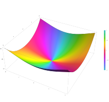
Plot of the Weber function E v(z) with n=2 in the complex plane from -2-2i to 2+2i with colors created with Mathematica 13.1 function ComplexPlot3D
sin ( π ν ) J ν ( z ) = cos ( π ν ) E ν ( z ) E ν ( z ) , sin ( π ν ) E ν ( z ) = cos ( π ν ) J ν ( z ) J ν ( z ) , {\displaystyle {\begin{aligned}\sin(\pi \nu )\mathbf {J} _{\nu }(z)&=\cos(\pi \nu )\mathbf {E} _{\nu }(z)-\mathbf {E} _{-\nu }(z),\\-\sin(\pi \nu )\mathbf {E} _{\nu }(z)&=\cos(\pi \nu )\mathbf {J} _{\nu }(z)-\mathbf {J} _{-\nu }(z),\end{aligned}}}

so in particular if ν is not an integer they can be expressed as linear combinations of each other. If ν is an integer then Anger functions Jν are the same as Bessel functions Jν, and Weber functions can be expressed as finite linear combinations of Struve functions.

Power series expansion

The Anger function has the power series expansion[2]

J ν ( z ) = cos π ν 2 k = 0 ( 1 ) k z 2 k 4 k Γ ( k + ν 2 + 1 ) Γ ( k ν 2 + 1 ) + sin π ν 2 k = 0 ( 1 ) k z 2 k + 1 2 2 k + 1 Γ ( k + ν 2 + 3 2 ) Γ ( k ν 2 + 3 2 ) . {\displaystyle \mathbf {J} _{\nu }(z)=\cos {\frac {\pi \nu }{2}}\sum _{k=0}^{\infty }{\frac {(-1)^{k}z^{2k}}{4^{k}\Gamma \left(k+{\frac {\nu }{2}}+1\right)\Gamma \left(k-{\frac {\nu }{2}}+1\right)}}+\sin {\frac {\pi \nu }{2}}\sum _{k=0}^{\infty }{\frac {(-1)^{k}z^{2k+1}}{2^{2k+1}\Gamma \left(k+{\frac {\nu }{2}}+{\frac {3}{2}}\right)\Gamma \left(k-{\frac {\nu }{2}}+{\frac {3}{2}}\right)}}.}

While the Weber function has the power series expansion[2]

E ν ( z ) = sin π ν 2 k = 0 ( 1 ) k z 2 k 4 k Γ ( k + ν 2 + 1 ) Γ ( k ν 2 + 1 ) cos π ν 2 k = 0 ( 1 ) k z 2 k + 1 2 2 k + 1 Γ ( k + ν 2 + 3 2 ) Γ ( k ν 2 + 3 2 ) . {\displaystyle \mathbf {E} _{\nu }(z)=\sin {\frac {\pi \nu }{2}}\sum _{k=0}^{\infty }{\frac {(-1)^{k}z^{2k}}{4^{k}\Gamma \left(k+{\frac {\nu }{2}}+1\right)\Gamma \left(k-{\frac {\nu }{2}}+1\right)}}-\cos {\frac {\pi \nu }{2}}\sum _{k=0}^{\infty }{\frac {(-1)^{k}z^{2k+1}}{2^{2k+1}\Gamma \left(k+{\frac {\nu }{2}}+{\frac {3}{2}}\right)\Gamma \left(k-{\frac {\nu }{2}}+{\frac {3}{2}}\right)}}.}

Differential equations

The Anger and Weber functions are solutions of inhomogeneous forms of Bessel's equation

z 2 y + z y + ( z 2 ν 2 ) y = 0. {\displaystyle z^{2}y^{\prime \prime }+zy^{\prime }+(z^{2}-\nu ^{2})y=0.}

More precisely, the Anger functions satisfy the equation[2]

z 2 y + z y + ( z 2 ν 2 ) y = ( z ν ) sin ( π ν ) π , {\displaystyle z^{2}y^{\prime \prime }+zy^{\prime }+(z^{2}-\nu ^{2})y={\frac {(z-\nu )\sin(\pi \nu )}{\pi }},}

and the Weber functions satisfy the equation[2]

z 2 y + z y + ( z 2 ν 2 ) y = z + ν + ( z ν ) cos ( π ν ) π . {\displaystyle z^{2}y^{\prime \prime }+zy^{\prime }+(z^{2}-\nu ^{2})y=-{\frac {z+\nu +(z-\nu )\cos(\pi \nu )}{\pi }}.}

Recurrence relations

The Anger function satisfies this inhomogeneous form of recurrence relation[2]

z J ν 1 ( z ) + z J ν + 1 ( z ) = 2 ν J ν ( z ) 2 sin π ν π . {\displaystyle z\mathbf {J} _{\nu -1}(z)+z\mathbf {J} _{\nu +1}(z)=2\nu \mathbf {J} _{\nu }(z)-{\frac {2\sin \pi \nu }{\pi }}.}

While the Weber function satisfies this inhomogeneous form of recurrence relation[2]

z E ν 1 ( z ) + z E ν + 1 ( z ) = 2 ν E ν ( z ) 2 ( 1 cos π ν ) π . {\displaystyle z\mathbf {E} _{\nu -1}(z)+z\mathbf {E} _{\nu +1}(z)=2\nu \mathbf {E} _{\nu }(z)-{\frac {2(1-\cos \pi \nu )}{\pi }}.}

Delay differential equations

The Anger and Weber functions satisfy these homogeneous forms of delay differential equations[2]

J ν 1 ( z ) J ν + 1 ( z ) = 2 z J ν ( z ) , {\displaystyle \mathbf {J} _{\nu -1}(z)-\mathbf {J} _{\nu +1}(z)=2{\dfrac {\partial }{\partial z}}\mathbf {J} _{\nu }(z),}
E ν 1 ( z ) E ν + 1 ( z ) = 2 z E ν ( z ) . {\displaystyle \mathbf {E} _{\nu -1}(z)-\mathbf {E} _{\nu +1}(z)=2{\dfrac {\partial }{\partial z}}\mathbf {E} _{\nu }(z).}

The Anger and Weber functions also satisfy these inhomogeneous forms of delay differential equations[2]

z z J ν ( z ) ± ν J ν ( z ) = ± z J ν 1 ( z ) ± sin π ν π , {\displaystyle z{\dfrac {\partial }{\partial z}}\mathbf {J} _{\nu }(z)\pm \nu \mathbf {J} _{\nu }(z)=\pm z\mathbf {J} _{\nu \mp 1}(z)\pm {\frac {\sin \pi \nu }{\pi }},}
z z E ν ( z ) ± ν E ν ( z ) = ± z E ν 1 ( z ) ± 1 cos π ν π . {\displaystyle z{\dfrac {\partial }{\partial z}}\mathbf {E} _{\nu }(z)\pm \nu \mathbf {E} _{\nu }(z)=\pm z\mathbf {E} _{\nu \mp 1}(z)\pm {\frac {1-\cos \pi \nu }{\pi }}.}

References

  1. ^ Prudnikov, A.P. (2001) [1994], "Anger function", Encyclopedia of Mathematics, EMS Press
  2. ^ a b c d e f g h Paris, R. B. (2010), "Anger-Weber Functions", in Olver, Frank W. J.; Lozier, Daniel M.; Boisvert, Ronald F.; Clark, Charles W. (eds.), NIST Handbook of Mathematical Functions, Cambridge University Press, ISBN 978-0-521-19225-5, MR 2723248.
  • Abramowitz, Milton; Stegun, Irene Ann, eds. (1983) [June 1964]. "Chapter 12". Handbook of Mathematical Functions with Formulas, Graphs, and Mathematical Tables. Applied Mathematics Series. Vol. 55 (Ninth reprint with additional corrections of tenth original printing with corrections (December 1972); first ed.). Washington D.C.; New York: United States Department of Commerce, National Bureau of Standards; Dover Publications. p. 498. ISBN 978-0-486-61272-0. LCCN 64-60036. MR 0167642. LCCN 65-12253.
  • C.T. Anger, Neueste Schr. d. Naturf. d. Ges. i. Danzig, 5 (1855) pp. 1–29
  • Prudnikov, A.P. (2001) [1994], "Weber function", Encyclopedia of Mathematics, EMS Press
  • G.N. Watson, "A treatise on the theory of Bessel functions", 1–2, Cambridge Univ. Press (1952)
  • H.F. Weber, Zurich Vierteljahresschrift, 24 (1879) pp. 33–76