Kurvenintegral

Das Kurven-, Linien-, Weg- oder Konturintegral erweitert den gewöhnlichen Integralbegriff für die Integration in der komplexen Ebene (Funktionentheorie) oder im mehrdimensionalen Raum (Vektoranalysis).

Den Weg, die Linie oder die Kurve, über die integriert wird, nennt man den Integrationsweg.

Wegintegrale über geschlossene Kurven werden auch als Ringintegral, Umlaufintegral^[1] oder Zirkulation bezeichnet und mit dem Symbol ${\displaystyle \textstyle \oint }$ geschrieben.

Das Wegintegral einer stetigen Funktion

${\displaystyle f\colon \mathbb {R} ^{n}\rightarrow \mathbb {R} }$

entlang eines stückweise stetig differenzierbaren Weges

${\displaystyle \gamma \colon [a,b]\to \mathbb {R} ^{n}}$

ist definiert als

${\displaystyle \int \limits _{\gamma }\!f\,\mathrm {d} s:=\int \limits _{a}^{b}\!f(\gamma (t))\,\|{\dot {\gamma }}(t)\|_{2}\,\mathrm {d} t.}$

Dabei bezeichnet ${\displaystyle {\dot {\gamma }}}$ die Ableitung von ${\displaystyle \gamma }$ nach ${\displaystyle t}$ und ${\displaystyle \|{\dot {\gamma }}(t)\|_{2}}$ die euklidische Norm des Vektors ${\displaystyle {\dot {\gamma }}(t)}$.

Die Bildmenge ${\displaystyle {\mathcal {C}}:=\gamma ([a,b])}$ ist eine stückweise glatte Kurve in ${\displaystyle \mathbb {R} ^{n}}$.

• Ein Beispiel für eine solche Funktion ${\displaystyle f}$ ist ein Skalarfeld mit kartesischen Koordinaten.
• Ein Weg ${\displaystyle \gamma }$ kann eine Kurve ${\displaystyle {\mathcal {C}}}$ entweder als Ganzes oder auch nur in Abschnitten mehrfach durchlaufen.
• Für ${\displaystyle f\equiv 1}$ ergibt das Wegintegral erster Art die Länge des Weges ${\displaystyle \gamma }$.
• Der Weg ${\displaystyle \gamma }$ bildet u. a. ${\displaystyle a\in \mathbb {R} }$ auf den Anfangspunkt der Kurve ab und ${\displaystyle b\in \mathbb {R} }$ auf deren Endpunkt.
• ${\displaystyle t\in [a,b]}$ ist ein Element der Definitionsmenge von ${\displaystyle \gamma }$ und steht allgemein nicht für die Zeit. ${\displaystyle \mathrm {d} t}$ ist das zugehörige Differential.

Das Wegintegral über ein stetiges Vektorfeld

${\displaystyle \mathbf {f} \colon \mathbb {R} ^{n}\rightarrow \mathbb {R} ^{n}}$

mit einer ebenfalls so parametrisierten Kurve ist definiert als das Integral über das Skalarprodukt aus ${\displaystyle \mathbf {f} \circ \gamma }$ und ${\displaystyle {\dot {\gamma }}}$:

${\displaystyle \int \limits _{\gamma }\!\mathbf {f} (\mathbf {x} )\cdot \mathrm {d} \mathbf {x} :=\int \limits _{a}^{b}\!\mathbf {f} (\gamma (t))\cdot {\dot {\gamma }}(t)\,\mathrm {d} t}$

Sind ${\displaystyle \gamma \colon [a,b]\to \mathbb {R} ^{n}}$ und ${\displaystyle \eta \colon [c,d]\to \mathbb {R} ^{n}}$ einfache (d. h., ${\displaystyle \gamma _{|(a,b)}}$ und ${\displaystyle \eta _{|(c,d)}}$ sind injektiv) Wege mit ${\displaystyle \gamma (a)=\eta (c)}$ und ${\displaystyle \gamma (b)=\eta (d)}$ und demselben Bild, parametrisieren sie also dieselbe Kurve in derselben Richtung und durchlaufen sie die Kurve (bis auf Doppelpunkte) genau einmal, so stimmen die Integrale entlang ${\displaystyle \gamma }$ und ${\displaystyle \eta }$ überein. Dies rechtfertigt den Namen Kurvenintegral; ist die Integrationsrichtung aus dem Kontext ersichtlich oder irrelevant, kann der Weg in der Notation unterdrückt werden.

Da eine Kurve ${\displaystyle {\mathcal {C}}}$ das Bild eines Weges ${\displaystyle \gamma }$ ist, entsprechen die Definitionen der Kurvenintegrale im Wesentlichen den Wegintegralen.

Kurvenintegral 1. Art:

${\displaystyle \int \limits _{\mathcal {C}}\!f\,\mathrm {d} s:=\int \limits _{a}^{b}\!f(\gamma (t))\|{\dot {\gamma }}(t)\|_{2}\,\mathrm {d} t}$

Kurvenintegral 2. Art:

${\displaystyle \int \limits _{\mathcal {C}}\mathbf {f} (\mathbf {x} )\cdot \mathrm {d} \mathbf {x} :=\int \limits _{a}^{b}\mathbf {f} (\gamma (t))\cdot {\dot {\gamma }}(t)\,\mathrm {d} t}$

Ein Spezialfall ist wieder die Länge der durch ${\displaystyle \gamma }$ parametrisierten Kurve ${\displaystyle {\mathcal {C}}}$:

${\displaystyle \mathrm {L{\ddot {a}}nge\ von\ } {\mathcal {C}}=\int \limits _{\mathcal {C}}\mathrm {d} s=\int \limits _{a}^{b}\|{\dot {\gamma }}(t)\|_{2}\,\mathrm {d} t}$

Der in den Kurvenintegralen erster Art auftretende Ausdruck

${\displaystyle \mathrm {d} s=\|{\dot {\gamma }}(t)\|_{2}\,\mathrm {d} t}$

heißt skalares Wegelement oder Längenelement. Der in den Kurvenintegralen zweiter Art auftretende Ausdruck

${\displaystyle \mathrm {d} \mathbf {x} ={\dot {\gamma }}(t)\,\mathrm {d} t}$

heißt vektorielles Wegelement.

Seien ${\displaystyle \int \limits _{\gamma }\mathbf {f} (\mathbf {x} )}$, ${\displaystyle \int \limits _{\gamma }\mathbf {g} (\mathbf {x} )}$ Kurvenintegrale gleicher Art (also entweder beide erster oder beide zweiter Art), sei das Urbild der beiden Funktionen ${\displaystyle \mathbf {f} }$ und ${\displaystyle \mathbf {g} }$ von gleicher Dimension und sei ${\displaystyle \gamma \colon [a,b]\to \mathbb {R} ^{n}}$. Dann gelten für ${\displaystyle \alpha }$, ${\displaystyle \beta \in \mathbb {R} }$ und ${\displaystyle c\in \mathbb {[} a,b]}$ die folgenden Rechenregeln:

• ${\displaystyle \alpha \int \limits _{\gamma }\mathbf {f} (\mathbf {x} )+\beta \int \limits _{\gamma }\mathbf {g} (\mathbf {x} )=\int \limits _{\gamma }(\alpha \mathbf {f} (\mathbf {x} )+\beta \mathbf {g} (\mathbf {x} ))}$    (Linearität)

• ${\displaystyle \int \limits _{\gamma }\mathbf {f} (\mathbf {x} )=\int \limits _{\gamma |_{[a,c]}}\mathbf {f} (\mathbf {x} )+\int \limits _{\gamma |_{[c,b]}}\mathbf {f} (\mathbf {x} )}$    (Zerlegungsadditivität)

Ist ${\displaystyle \gamma }$ ein geschlossener Weg, so schreibt man

statt ${\displaystyle \displaystyle \int \limits _{\gamma }}$ auch ${\displaystyle \displaystyle \oint \limits _{\gamma }}$

und analog für geschlossene Kurven ${\displaystyle {\mathcal {C}}}$

statt ${\displaystyle \displaystyle \int \limits _{\mathcal {C}}}$ auch ${\displaystyle \displaystyle \oint \limits _{\mathcal {C}}}$.

Mit dem Kreis im Integral möchte man deutlich machen, dass ${\displaystyle \gamma }$ geschlossen ist. Der einzige Unterschied liegt hierbei in der Notation.

• Ist ${\displaystyle {\mathcal {C}}}$ der Graph einer Funktion ${\displaystyle f\colon [a,b]\to \mathbb {R} }$, so wird diese Kurve durch den Weg

${\displaystyle \gamma \colon [a,b]\to \mathbb {R} ^{2},\quad t\mapsto (t,f(t))}$

parametrisiert. Wegen

${\displaystyle \|{\dot {\gamma }}(t)\|_{2}={\sqrt {1+f'(t)^{2}}}}$

ist die Länge der Kurve gleich

${\displaystyle \int \limits _{\mathcal {C}}\mathrm {d} s=\int \limits _{a}^{b}{\sqrt {1+f'(t)^{2}}}\,\mathrm {d} t.}$

• Eine Ellipse mit großer Halbachse ${\displaystyle a}$ und kleiner Halbachse ${\displaystyle b}$ wird durch ${\displaystyle (a\cos t,\,b\sin t)}$ für ${\displaystyle t\in [0,2\pi ]}$ parametrisiert. Ihr Umfang ist also

${\displaystyle \int \limits _{0}^{2\pi }{\sqrt {a^{2}\sin ^{2}t+b^{2}\cos ^{2}t}}\,\mathrm {d} t=4a\int \limits _{0}^{\frac {\pi }{2}}{\sqrt {1-\varepsilon ^{2}\cos ^{2}t}}\;\mathrm {d} t}$.

Dabei bezeichnet ${\displaystyle \varepsilon }$ die numerische Exzentrizität ${\displaystyle {\sqrt {1-b^{2}/a^{2}}}}$ der Ellipse. Das Integral auf der rechten Seite wird aufgrund dieses Zusammenhanges als elliptisches Integral bezeichnet.

Ist ein Vektorfeld ${\displaystyle \mathbf {F} }$ ein Gradientenfeld, d. h., ${\displaystyle \mathbf {F} }$ ist der Gradient eines skalaren Feldes ${\displaystyle V}$, mit

${\displaystyle \mathbf {\nabla } V=\mathbf {F} }$,

so gilt für die Ableitung der Verkettung von ${\displaystyle V}$ und ${\displaystyle \mathbf {r} (t)}$

${\displaystyle {\frac {\mathrm {d} }{\mathrm {d} t}}V(\mathbf {r} (t))=\mathbf {\nabla } V(\mathbf {r} (t))\cdot {\dot {\mathbf {r} }}(t)=\mathbf {F} (\mathbf {r} (t))\cdot {\dot {\mathbf {r} }}(t)}$,

was gerade dem Integranden des Wegintegrals über ${\displaystyle \mathbf {F} }$ auf ${\displaystyle \mathbf {r} (t)}$ entspricht. Daraus folgt für eine gegebene Kurve ${\displaystyle {\mathcal {S}}}$

${\displaystyle \int \limits _{\mathcal {S}}\mathbf {F} (\mathbf {x} )\cdot \,\mathrm {d} \mathbf {x} =\int \limits _{a}^{b}\mathbf {F} (\mathbf {r} (t))\cdot {\dot {\mathbf {r} }}(t)\,\mathrm {d} t=\int \limits _{a}^{b}{\frac {\mathrm {d} }{\mathrm {d} t}}V(\mathbf {r} (t))\,\mathrm {d} t=V(\mathbf {r} (b))-V(\mathbf {r} (a)).}$

Dies bedeutet, dass das Integral von ${\displaystyle \mathbf {F} }$ über ${\displaystyle {\mathcal {S}}}$ ausschließlich von den Punkten ${\displaystyle \mathbf {r} (b)}$ und ${\displaystyle \mathbf {r} (a)}$ abhängt und der Weg dazwischen irrelevant für das Ergebnis ist. Aus diesem Grund wird das Integral eines Gradientenfeldes als „wegunabhängig“ bezeichnet.

Insbesondere gilt für das Ringintegral über die geschlossene Kurve ${\displaystyle {\mathcal {S}}}$ mit zwei beliebigen Wegen ${\displaystyle {\mathcal {S}}_{1}}$ und ${\displaystyle {\mathcal {S}}_{2}}$:

${\displaystyle \oint \limits _{\mathcal {S}}\mathbf {F} (\mathbf {x} )\,\mathrm {d} \mathbf {x} =\int \limits _{1,{\mathcal {S}}_{1}}^{2}\mathbf {F} (\mathbf {x} )\,\mathrm {d} \mathbf {x} +\int \limits _{2,{\mathcal {S}}_{2}}^{1}\mathbf {F} (\mathbf {x} )\,\mathrm {d} \mathbf {x} =0}$

Dies ist insbesondere in der Physik von großer Bedeutung, da beispielsweise die Gravitation diese Eigenschaften besitzt. Da die Energie in diesen Kraftfeldern stets eine Erhaltungsgröße ist, werden sie in der Physik als konservative Kraftfelder bezeichnet. Das skalare Feld ${\displaystyle V}$ ist dabei das Potential oder die potentielle Energie. Konservative Kraftfelder erhalten die mechanische Energie, d. i. die Summe aus kinetischer Energie und potentieller Energie. Gemäß dem obigen Integral wird auf einer geschlossenen Kurve insgesamt eine Arbeit von 0 J aufgebracht.

Wegunabhängigkeit lässt sich auch mit Hilfe der Integrabilitätsbedingung zeigen.

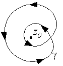
Ist das Vektorfeld nur in einer (kleinen) Umgebung ${\displaystyle U}$ eines Punktes nicht als Gradientenfeld darstellbar, so ist das geschlossene Wegintegral von Kurven außerhalb von ${\displaystyle U}$ proportional zur Windungszahl um diesen Punkt und ansonsten unabhängig vom genauen Verlauf der Kurve (siehe Algebraische Topologie: Methodik).

Ist ${\displaystyle f\colon [a,b]\to \mathbb {C} }$ eine komplexwertige Funktion, dann nennt man ${\displaystyle f}$ integrierbar, wenn ${\displaystyle \operatorname {Re} f}$ und ${\displaystyle \operatorname {Im} f}$ integrierbar sind. Man definiert

${\displaystyle \int \limits _{a}^{b}f(x)\mathrm {d} x:=\int \limits _{a}^{b}\operatorname {Re} f(x)\mathrm {d} x+\mathrm {i} \int \limits _{a}^{b}\operatorname {Im} f(x)\mathrm {d} x}$.

Das Integral ist damit ${\displaystyle \mathbb {C} }$-linear. Ist ${\displaystyle f}$ im Intervall ${\displaystyle [a,b]}$ stetig und ${\displaystyle F}$ eine Stammfunktion von ${\displaystyle f}$, so gilt wie im Reellen

${\displaystyle \int \limits _{a}^{b}f(x)\mathrm {d} x=F(b)-F(a)}$.

Der Integralbegriff wird nun auf die komplexe Ebene wie folgt erweitert: Ist ${\displaystyle f\colon U\to \mathbb {C} }$ eine komplexwertige Funktion auf einem Gebiet ${\displaystyle U\subseteq \mathbb {C} }$, und ist ${\displaystyle \gamma \colon [0,1]\to U}$ ein stückweise stetig differenzierbarer Weg in ${\displaystyle U}$, so ist das Wegintegral von ${\displaystyle f}$ entlang des Weges ${\displaystyle \gamma }$ definiert als

${\displaystyle \int \limits _{\gamma }f:=\int \limits _{\gamma }f(z)\,\mathrm {d} z:=\int \limits _{0}^{1}f(\gamma (t))\cdot {\dot {\gamma }}(t)\,\mathrm {d} t.}$

Der Malpunkt bezeichnet hier komplexe Multiplikation.

Die zentrale Aussage über Wegintegrale komplexer Funktionen ist der Cauchysche Integralsatz: Für eine holomorphe Funktion ${\displaystyle f}$ hängt das Wegintegral nur von der Homotopieklasse von ${\displaystyle \gamma }$ ab. Ist ${\displaystyle U}$ einfach zusammenhängend, so hängt das Integral also überhaupt nicht von ${\displaystyle \gamma }$, sondern nur von Anfangs- und Endpunkt ab.

Analog zum reellen Fall definiert man die Länge des Weges ${\displaystyle \gamma }$ durch

${\displaystyle \operatorname {L} (\gamma ):=\int \limits _{0}^{1}\left|{\dot {\gamma }}(t)\right|\mathrm {d} t}$.

Für theoretische Zwecke ist folgende Ungleichung, die Standardabschätzung, von besonderem Interesse:

${\displaystyle \left|\int _{\gamma }f(z)\,\mathrm {d} z\right|\leq \operatorname {L} (\gamma )\cdot C}$, wenn ${\displaystyle \left|f(z)\right|\leq C}$ für alle ${\displaystyle z\in \gamma ([0,1])}$ gilt.

Wie im reellen Fall ist das Wegintegral unabhängig von der Parametrisierung des Weges ${\displaystyle \gamma }$, d. h., es ist nicht zwingend notwendig, ${\displaystyle [0,1]}$ als Parameterbereich zu wählen, wie sich durch Substitution zeigen lässt. Dies erlaubt die Definition komplexer Kurvenintegrale, indem man den obigen Formeln den Weg ${\displaystyle \gamma }$ durch eine Kurve ${\displaystyle {\mathcal {C}}}$ in ${\displaystyle \mathbb {C} }$ ersetzt.

• Pfadintegral

• Harro Heuser: Lehrbuch der Analysis – Teil 2. 1981, 5. Auflage, Teubner 1990, ISBN 3-519-42222-0. S. 369, Satz 180.1; S. 391, Satz 184.1; S. 393, Satz 185.1.

• Kurvenintegrale bei Matroids Matheplanet

1. ↑ Klaus Knothe, Heribert Wessels: Finite Elemente. Eine Einführung für Ingenieure. 3. Auflage. 1999, ISBN 3-540-64491-1, S. 524.